Linear correlation

Attention

Finnish university students are encouraged to use the CSC Noppe platform.

Others can follow the lesson and fill in their student notebooks using Binder.

In many cases, we might expect our data to have some kind of relationship, such as that between the temperature at which magma erupts and the SiO₂ content of the magma, as shown back in Figure 1 in the least-squares part of the lesson. The correlation between two variables can be assessed using the correlation coefficient \(r\), also known as the Pearson correlation coefficient. \(r\) ranges between -1 to 1, with a value of 1 reflecting data that perfectly fit a line with a positive slope, a value of -1 representing data that perfectly fit a line with a negative slope, and a value around 0 representing data that either are not correlated or do not fit a straight line. You can find a number of different correlation coefficients below in Figure 2.2.

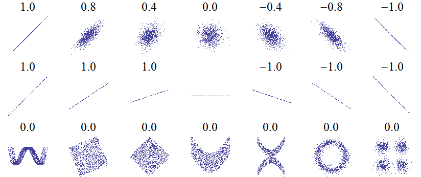
Figure 2.2. Examples of Pearson correlation coefficients for different data point distributions. Source: https://commons.wikimedia.org/wiki/File:Correlation_examples.png.

Calculating the correlation coefficient

Mathematically, we can define the correlation coefficient \(r\) as

\[ \large r = \frac{\sum{\left(x_{i} - \bar{x} \right)\left(y_{i} - \bar{y} \right)}}{\sqrt{\sum{\left(x_{i} - \bar{x} \right)^2} \sum{\left(y_{i} - \bar{y} \right)^2}}}, \]

where \(x_{i}\) is the \(i\)th value along the \(x\)-axis, \(\bar{x}\) is the mean of the values on the \(x\)-axis, and similarly for the values of \(y\). Using the equation above, we can calculate \(r\), which measures how well the data \(x\) and \(y\) are linearly related.