Lesson 3 demonstration notebook#
while loops in Python#
A while loop in Python can be used to iterate in a loop until a certain condition is met. In the example below we iterate until the name Uncle Ismo is encountered.
names = ['Dave', 'Leevi', 'Uncle Ismo', 'Woofy']

name_index = 0
while names[name_index] != 'Uncle Ismo':
    print(names[name_index])
    name_index = name_index + 1
Dave
Leevi
For certain kinds of “iterative” problems, it can be better to use a while loop than a for loop to run a calculation until a “converged” solution is found.
The example below is a code that finds the square root of an input number starting from an initial guess. An example with a for loop is shown first, and then the equivalent calculation using a while loop. I have modified the numbers from the example in the lesson video so that the same number and guess are used in both examples. You will notice that fewer iterations are used in the while loop case because the calculation stops once the solution for estimate of the square root is no longer changing.
number = 142344
guess = 72234

for i in range(20):
    guess = 0.5 * (guess + number / guess)
    #print(guess)

print(f"The square root of {number} is {guess} after {i+1} iterations.")
The square root of 142344 is 377.2850381342997 after 20 iterations.
number = 142344
guess = 72234
guess_diff = 1.0

counter = 0
while guess_diff > 0.0000001:
    counter = counter + 1
    guess_orig = guess
    guess = 0.5 * (guess + number / guess)
    guess_diff = abs(guess_orig - guess)

print(f"The square root of {number} is {guess} after {counter} iterations.")
The square root of 142344 is 377.2850381342997 after 13 iterations.
Logarithmic scaling and plot axes#
The other point we discussed was related to using a logarithmic scale on one or more of the plot axes and how to maintain a uniform spacing between points used for calculations.
First, we created two NumPy arrays with values going from 0.01 to 100.0 either with linear (x) or logarithmic (´x2´) spacing between values.
import numpy as np
import matplotlib.pyplot as plt
x = np.linspace(0.01, 100.0, 11)
x
array([1.0000e-02, 1.0009e+01, 2.0008e+01, 3.0007e+01, 4.0006e+01,
       5.0005e+01, 6.0004e+01, 7.0003e+01, 8.0002e+01, 9.0001e+01,
       1.0000e+02])
x2 = np.logspace(-2, 2, 11)
x2
array([1.00000000e-02, 2.51188643e-02, 6.30957344e-02, 1.58489319e-01,
       3.98107171e-01, 1.00000000e+00, 2.51188643e+00, 6.30957344e+00,
       1.58489319e+01, 3.98107171e+01, 1.00000000e+02])
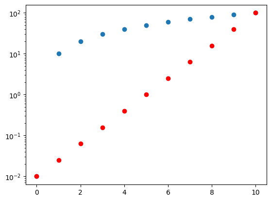
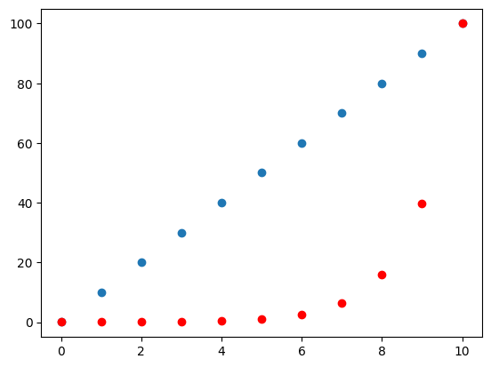
To visualize the difference in the spacing between the points we can look at two different plots of the values. The index of the points is on the x-axis, and the values themselves on the y-axis. In the first case, we have linear scalint of the points on the y-axis and you can see the points of x are equal, whereas the points in x2 are not.
fig, ax = plt.subplots(1, 1)

ax.plot(x, 'o')
ax.plot(x2, 'ro')
[<matplotlib.lines.Line2D at 0x768f4f345810>]
In contrast, when the y-axis has a logarithmic scale, the x2 points are now uniformly spaced and those in x are not. This can be important to ensure your plots have good representation of all values when visualizing the data.
fig, ax = plt.subplots(1, 1)

ax.plot(x, 'o')
ax.plot(x2, 'ro')
ax.set_yscale("log")